The Evolution of Robustness
by Wim Hordijk and Lee Altenberg
1 November 2019
In Darwin’s theory of evolution by natural selection, the key phrase is “survival of the fittest”: those organisms that are best fit to carry out the tasks of living in their world are the ones that survive. But they won’t live forever — they must have offspring that inherit the traits that made them fit in order for evolution to proceed.
This conceptual framework is fine for understanding the evolution of traits that affect survival and numbers of offspring. But what about the rules of inheritance themselves? These rules are also organismal traits, although they need not have any effect on how well the parents survive or how many offspring they have. In fact, the rules of inheritance say what the offspring are, rather than how many there are. Classical mathematical models of evolution have little to say about the evolution of these rules. How, then, can “survival of the fittest” shape the rules of inheritance?
Evolvability and robustness
One of the exciting developments in evolutionary theory since the Modern Synthesis has been the theory of how genes that control inheritance should themselves evolve (i.e., modifier gene theory, pioneered by Marc Feldman). Another new development in the extended evolutionary synthesis is theory on how changes to genes should map to changes in organisms (i.e., the theory of the evolution of the genotype-phenotype map). Two principal phenomena have emerged from this new theory: (1) the evolution of robustness, and (2) the evolution of evolvability.
Not only do organisms evolve to become better adapted to their environment, but the genes that encode these adaptations are predicted to become more robust against mutations. In other words, changes in genes between parents and offspring may not cause any significant change in an organism’s already well-adapted traits. Furthermore, those changes in traits that do occur may become focused on traits that can still be improved, while leaving alone those traits for which change is only destructive. The latter represents the evolution of evolvability, while the former represents the evolution of robustness.
Robustness can be defined in terms of the fraction of deleterious mutants. Imagine we could take an organism and produce and evaluate all its single-site mutants. We can then simply count the number of these mutants that have a lower fitness than the original organism. An organism with a smaller fraction of such deleterious mutants is more robust than an equally fit organism with a larger fraction of deleterious mutants.
As simple as this may sound, empirically it is difficult to implement with real organisms. So is it possible at all to measure, or even just observe, the evolution of robustness? To investigate this, computer models are a useful tool. In recent work we used cellular automata as models of developmental systems, and then applied a genetic algorithm to evolve these cellular automata to produce some non-trivial dynamical behavior. To our delight, the evolution of robustness could not only be clearly observed, but also quantitatively analyzed.
These results were recently published in an article in the journal Evolution & Development, as part of a special issue that resulted from the EES workshop on developmental biases in evolution which was held at the Santa Fe Institute last year. Here we present a brief and non-technical overview of some of our results.
Cellular automata
Beautiful, complex patterns in the biological world are understood to arise in many cases from simple, local interactions between cells and molecular components. Cellular automata are computational models that abstract the idea of simple local interactions, and are used to understand how such complex patterns can emerge from these bare elements.
In its most basic form, a cellular automaton (CA) consists of a linear array of “cells”, each of which can be in one of two states, say zero or one. At discrete time steps, or iterations, all cells simultaneously update their state. The new state of a cell depends on its current neighborhood configuration consisting of the states of the cell itself, its left neighbor, and its right neighbor. A fixed update rule then simply states for each possible local neighborhood configuration what the new state of the center cell will be.
Given two possible cell states and a three-cell neighborhood, there are thus 2x2x2=23=8 possible neighborhood configurations. An example of a CA update rule is given in the table below, with the eight possible neighborhood configurations given in the top row, and the corresponding new cell states in the bottom row.
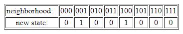
This most basic form of a CA is known as an elementary cellular automaton (ECA). The particular update rule shown in the table above is known as ECA 18. However, note that the bottom row (new cell states) could have had any assignment of zeros and ones. Thus, there are 28=256 possible ECA update rules. Depending on which particular rule is used, the system as a whole (i.e., the array of cells iterated over time) can show very different types of dynamical behavior, from fixed point or simple periodic to very complex or even seemingly random behavior.
The image above shows the dynamical behavior of ECA 18 in a so-called space-time diagram. White squares represent cells that are in state zero, while black squares represent cells in state one. In this diagram, space is horizontal (100 cells wide) and time is vertical (100 iterations down). The top row in the diagram is the initial configuration, which was generated at random. Each next row in the space-time diagram is the CA configuration after applying the update rule given in the table above to all cells simultaneously.
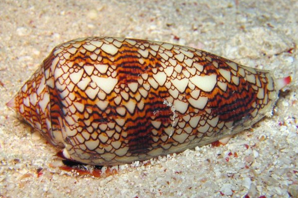
Interestingly, ECA 18 produces patterns that look very similar to those that can be observed on certain types of sea shells. These patterns are considered to be emergent. They form at a global scale, even though each individual cell in the CA can only interact locally with its direct neighbors (through the update rule). The global dynamics cannot be mathematically derived or predicted from just the local update rule, other than actually iterating the system over time.
One particular type of emergent pattern formation that is observed frequently in biological systems is that of synchronized oscillations. For example, fireflies flash on and off in synchrony, and synchronized oscillations can also be observed in neural assemblies, or in bacterial colonies. So, one could ask: Is there a CA update rule that produces such synchronized oscillations?
Clearly ECA 18 does not. In fact, neither do any of the other 255 ECA update rules. However, when we allow for a slightly more general update rule, for example by considering additional neighbors to determine a cell’s new state, the possible types of dynamical behaviors that can be produced also increases.
Consider a CA update rule where not just one neighbor to the left and right is considered, but three on either side. This gives rise to a neighborhood of seven cells (instead of three), resulting in 27=128 possible neighborhood configurations. In other words, the update rule now has 128 entries (instead of eight), each one having a zero or a one for the corresponding new cell state.
Could such a more general CA update rule produce synchronized oscillations? Unfortunately that question is much harder to answer. In fact, now there are 2128≈3.4×1038 possible update rules. This is an astronomically large number, and it is impossible to simply try every rule to see if it produces the desired behavior. However, taking another clue from nature, we can use a genetic algorithm to try to evolve such a rule.
Evolving synchronized oscillations
A genetic algorithm is a simple computer program that mimics natural evolution. It is often used to find good solutions to difficult optimization problems (see an earlier article about evolutionary algorithms). It can also be used to evolve cellular automata update rules to produce synchronized oscillations.
In such a genetic algorithm application, a CA’s update rule is considered the genotype, and the resulting dynamical behavior (as visualized in a space-time diagram) is the phenotype. The fitness (i.e., average or expected reproductive success) of a CA update rule is determined by its ability to generate the desired behavior. This is measured as the fraction of a given number (say 100) of random initial configurations on which the CA correctly produces synchronized oscillations. In other words, the better a CA is at generating the desired behavior, the more offspring it will have, on average.
The genetic algorithm then evolves an (initially random) population of CA update rules by repeatedly applying selection, recombination, and mutation on the current population to form subsequent generations. Indeed, such a process of simulated evolution does often result in CA update rules that produce the desired dynamical behavior.
The figure above shows several space-time diagrams of one particularly successful CA update rule that resulted from this genetic algorithm evolution. Each next image shows the dynamical behavior of the CA starting from a different (random) initial configuration. Note that periodic boundary conditions are used, where the leftmost and rightmost cells are each other’s neighbors (in other words, the array is considered to be circular).
In each space-time diagram, locally synchronized regions appear almost immediately (i.e., near the top of the image). However, often these local regions are out of phase with each other. For example, at one particular iteration (row) one such synchronized region may be in state zero (white), while another is in state one (black). The CA uses an additional pattern (the “zig-zag” regions), to resolve these phase conflicts, eventually ending up in a globally synchronized oscillation between all-white and all-black (towards the bottom of the image).
The evolution of robustness
Recall that robustness is defined in terms of the fraction of mutations that lead to a reduced fitness. An organism with a smaller fraction of such deleterious mutations is more robust than one with a larger fraction.
Using the results from our cellular automaton model, we can now study the evolution of robustness as follows. First, for each generation during the run of the genetic algorithm, we take the fittest CA update rule in the population. In other words, for each generation we take the CA that produces the desired synchronous oscillations on the largest fraction of random initial configurations. Next, we generate all single-site mutants of these best-in-generation CAs. And finally, we calculate the fitness of all these mutants and count how many have a fitness that is lower than that of the original CA.
What we found is that the robustness of the CAs tends to increase during their evolution, even when they are already well adapted, i.e., when there is no more increase in fitness.
In our experiments, the genetic algorithm was run for 100 generations. So, we have 100 best-in-generation CA rules, one from each generation. Now, recall that each CA update rule has 128 entries, with each entry containing either a zero or a one to indicate the new cell state. This means that each CA rule has 128 single-site mutants. Each such mutant is the original CA rule with one of the entries mutated, i.e., a zero changed to a one or vice versa.
Once we have all these 128 mutants of a best-in-generation CA rule, we can simply calculate the fitness of each of them in the same way: each mutant CA rule is iterated on a large set of random initial configurations, and the fraction on which it generates the desired synchronous oscillations is its fitness. Finally, we count how many of these mutants have a lower fitness than the best-in-generation CA itself, and express this as a fraction (i.e., we simply divide the number of deleterious mutants by 128).
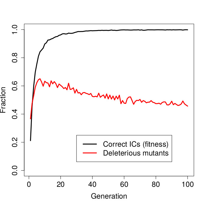
The figure above shows the result. On the horizontal axis in this graph are the genetic algorithm generations. The black curve shows the fitness (fraction of initial configurations on which synchronization was achieved) of the best-in-generation CAs over time. The red curve shows the fraction of deleterious mutants of these best-in-generation CAs.
First note that the fitness values quickly approach 1.0. After about 30 generations, the genetic algorithm has already evolved CA rules that produce the desired synchronous oscillations almost perfectly, i.e, on almost all (random) initial configurations.
However, while an almost perfect fitness has been reached by about generation 30, there is still selective pressure for the CA rules to become more robust. This is reflected in the red curve representing the fraction of deleterious mutants. Initially this fraction increases very rapidly, but then gradually declines over time. In other words, even though the CA rules are already well adapted (no more increase in fitness), they continue to evolve in terms of increased robustness.
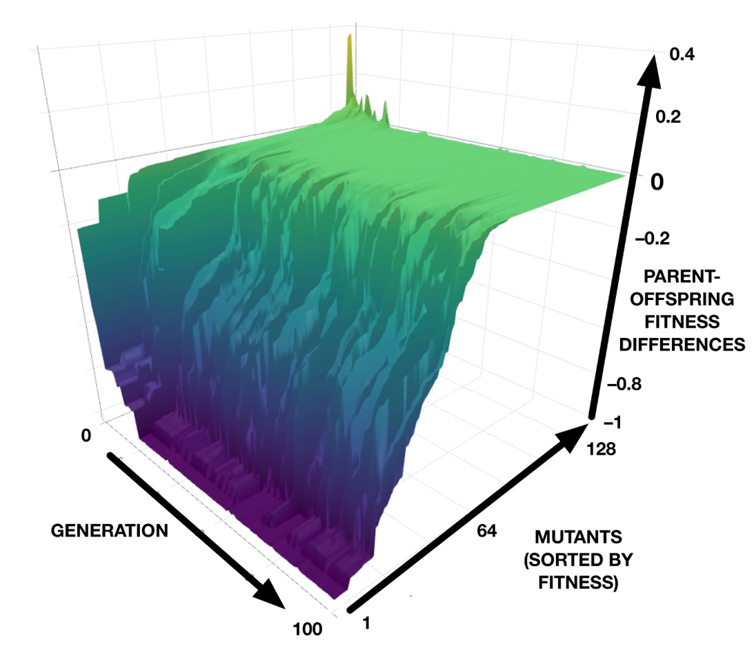
The results from our computer models can be investigated in even more detail. For example, we can plot the differences in fitness between a best-in-generation CA and each of its 128 mutants, for each generation in a genetic algorithm run. This results in a 3D plot that can be interpreted as a “mutational landscape”, as shown in the image below. The green plateau represents neutrality, while the purple “abyss” represents lethality. (See also an interactive version that can be zoomed and rotated.)

Earlier work on this CA model discovered that the synchronization task can be achieved by two very different developmental strategies: one, which we showed here, synchronizes most cells very quickly and then gradually eliminates the out-of-phase domains; the other, not shown here, takes long convoluted paths to synchronization. In the convoluted pathways, mutational robustness does not evolve; rather, as adaptation increases, the developmental pathways become even more complicated and their sensitivity to mutation remains high. This reveals that the evolution of mutational robustness is not a universal outcome, but depends on the nature of the developmental strategy that evolution discovered for the adaptation.
Even though these results come from computer models, they do show that the evolution of robustness is a real phenomenon, and that in principle it can be studied and analyzed quantitatively. Hopefully this will provide a stimulus for evolutionary and developmental biologists to try and observe, measure, and analyze this phenomenon in real organisms. Robustness clearly plays an important role in evolution. And computer models like the one described here provide a useful tool for studying its occurrence and role in more detail.